Columnar Storage - SoliDB Documentation

Overview

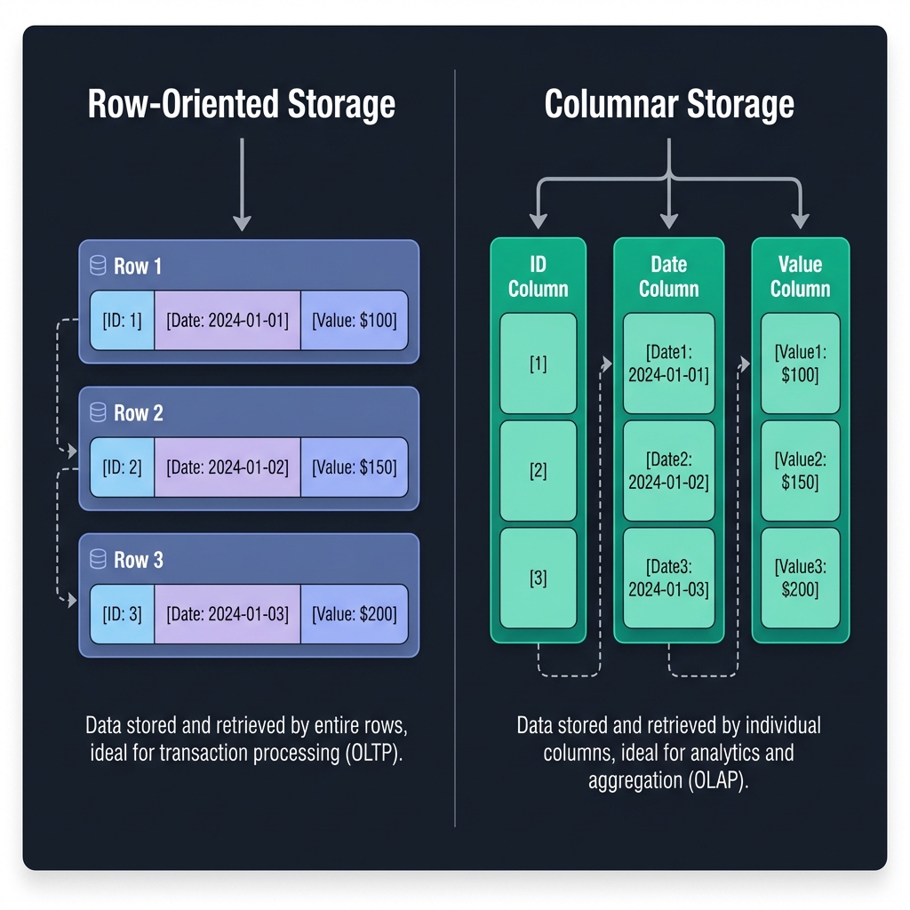
Unlike traditional row-oriented collections where data is stored document-by-document, columnar collections store data column-by-column. This architecture is vastly superior for analytical queries where you typically access only a few columns but scan millions of rows.

Compression

LZ4 compression often achieves 2-4x better storage efficiency than row storage.

Pruning

Read only the columns you need. IO is reduced proportionally to the number of columns skipped.

Grouping

Efficient GROUP BY and aggregation operations (SUM, AVG, MIN, MAX).

Typed

Explicit schemas with supported types: Int64, Float64, String, Bool, Timestamp, Json.

Columnar vs. Standard Time Series

SoliDB offers two distinct approaches for handling time-based data. Choosing the right one depends on your ingestion and query patterns.

Feature	Standard Time Series	Columnar Storage
Storage Layout	Row-oriented (Log Structured)	Column-oriented (Chunked)
Best For	High-throughput ingestion, real-time monitoring, simple retrieval	Complex analytics, reporting, aggregations over large history
Ingestion	Fast individual inserts & appends	Favors batched bulk inserts
Retention	TTL & Pruning supported	Manual management
Primary Ops	`INSERT`, `GET range`	`GROUP BY`, `SUM`, `AVG`

Recommendation: Use Time Series collections for raw data ingestion and real-time dashboards. Offload historical data to Columnar collections for long-term storage and heavy analytical reporting.

Creating Collections

Columnar collections require an explicit schema definition at creation time. This allows the engine to optimize storage layout.

POST /_api/database/:db/columnar

{
  "name": "server_metrics",
  "compression": "lz4",
  "columns": [
    { "name": "timestamp", "type": "TIMESTAMP" },
    { "name": "host", "type": "STRING" },
    { "name": "cpu_usage", "type": "FLOAT64" },
    { "name": "requests", "type": "INT64" },
    { "name": "metadata", "type": "JSON", "nullable": true }
  ]
}

INT64 FLOAT64 STRING BOOL TIMESTAMP JSON

Inserting Data

Insertions should ideally be batched for maximum performance. The engine automatically handles decomposition into columns and compression.

POST /_api/database/:db/columnar/:collection/insert

{
  "rows": [
    {
      "timestamp": "2024-01-01T10:00:00Z",
      "host": "us-east-1a",
      "cpu_usage": 45.2,
      "requests": 1024
    },
    {
      "timestamp": "2024-01-01T10:00:01Z",
      "host": "us-east-1a",
      "cpu_usage": 48.1,
      "requests": 1150
    }
  ]
}

Aggregations

Perform fast aggregations on single columns or with grouping. The engine reads only the necessary columns and uses streaming processing for minimal memory footprint (O(1)).

Simple Aggregate

Calculate metrics across the entire collection.

SDBQL

FOR c IN cpu_logs
  COLLECT AGGREGATE
    avg_usage = AVG(c.usage)
  RETURN { avg_usage }

API

{
  "column": "usage",
  "operation": "AVG"
}

Group By

Group results by one or more columns.

SDBQL

FOR r IN requests
  COLLECT
    host = r.host
  AGGREGATE
    total = SUM(r.count)
  RETURN { host, total }

API

{
  "column": "count",
  "operation": "SUM",
  "group_by": ["host"]
}

Time Bucket

Group by fixed time intervals (e.g., 1h, 5m). Optimized for time-series.

SDBQL

FOR m IN metrics
  COLLECT
    time = TIME_BUCKET(m.ts, '1h'),
    host = m.host
  AGGREGATE
    avg_cpu = AVG(m.cpu)
  RETURN { time, host, avg_cpu }

API

{
  "column": "cpu",
  "operation": "AVG",
  "group_by": ["TIME_BUCKET(ts, '1h')", "host"]
}
// Note: SDBQL is recommended for this

Supported Operations

SUM AVG COUNT MIN MAX COUNT_DISTINCT

Filtering & Querying

Query raw data with column projection and filtering. Filters are applied before projection to minimize IO.

POST /_api/database/:db/columnar/:collection/query

{
  "columns": ["timestamp", "cpu_usage"],
  "filter": {
    "column": "host",
    "op": "EQ",
    "value": "us-east-1a"
  },
  "limit": 100
}

Filter Operators

EQ (=) NE (!=) GT (>) GTE (>=) LT (<) LTE (<=) IN

Advanced Indexing

SoliDB supports advanced columnar index types to accelerate specific query patterns. Indexes are created independently of the data and can be added or removed at any time.

Bitmap Index

Best for low-cardinality columns (e.g., status, category, boolean flags). Uses highly compressed bitsets (LZ4) to perform blazing fast equality and IN lookups.

Type: "bitmap" Ideal for: < 100 distinct values

Min/Max Index

Best for range queries on sorted or semi-sorted data (e.g., timestamps, sequential IDs). Divides data into chunks and skips entire blocks that don't match the filter (Partition Pruning).

Type: "minmax" Overhead: Ultra-low (~0.1%)

Hash Index

Best for exact match queries (equality) on high-cardinality columns (e.g., UUIDs, user IDs). O(1) lookups but does not support range queries.

Type: "hash" Fastest for: Equality

Bloom Filter Index

Best for probabilistic membership testing. Checks if a value might exist in a chunk before scanning it. Useful for skipping chunks for equality checks on unique or semi-unique columns.

Type: "bloom" No False Negatives

Sorted Index (Default)

Standard index storing a sorted list of values pointing to list of Row IDs. Good general purpose performance for both equality and range queries on high-cardinality data.

POST /_api/database/:db/columnar/:collection/index

{
  "column": "status",
  "index_type": "bitmap"
}

IoT & Sensor Data

Store high-frequency sensor readings from thousands of devices. Use Time Bucket aggregations to downsample data for visualization (e.g., convert 1-second resolution to 5-minute averages).

SDBQL

FOR s IN sensors
  FILTER s.region == 'us-east-1'
  COLLECT
    bucket = TIME_BUCKET(s.ts, '5m'),
    device = s.device_id
  AGGREGATE
    avg_temp = AVG(s.temperature),
    max_temp = MAX(s.temperature),
    avg_humidity = AVG(s.humidity)
  RETURN { 
    time: bucket, 
    device, 
    temp: avg_temp, 
    max: max_temp, 
    humidity: avg_humidity 
  }

Financial Analytics

Analyze trade data to produce OHLCV (Open, High, Low, Close, Volume) candles and VWAP (Volume Weighted Average Price) efficiently.

SDBQL

FOR t IN trades
  COLLECT
    bucket = TIME_BUCKET(t.ts, '1m'),
    symbol = t.symbol
  AGGREGATE
    open = FIRST(t.price),
    high = MAX(t.price),
    low = MIN(t.price),
    close = LAST(t.price),
    volume = SUM(t.size),
    vwap_num = SUM(t.price * t.size)
  RETURN { 
    time: bucket, 
    symbol, 
    open, high, low, close, volume,
    vwap: vwap_num / volume 
  }